Matrices

Since this is a guide on graphics programming, this chapter will not cover a lot of the extensive theory behind matrices. Only the theory that applies to their use in computer graphics will be considered here and they will be explained from a programmer's perspective. If you want to learn more about the topic, these Khan Academy videos are a really good general introduction to the subject.

A matrix is a rectangular array of mathematical expressions, much like a two-dimensional array. Below is an example of a matrix displayed in the common square brackets form.

Matrices values are indexed by (i,j) where i is the row and j is the column. That is why the matrix displayed above is called a 3-by-2 matrix. To refer to a specific value in the matrix, for example 5, the $a_{31}$ notation is used.

Basic operations

To get a bit more familiar with the concept of an array of numbers, let's first look at a few basic operations.

Addition and subtraction

Just like regular numbers, the addition and subtraction operators are also defined for matrices. The only requirement is that the two operands have exactly the same row and column dimensions.

The values in the matrices are individually added or subtracted from each other.

Scalar product

The product of a scalar and a matrix is as straightforward as addition and subtraction.

The values in the matrices are each multiplied by the scalar.

Matrix-Vector product

The product of a matrix with another matrix is quite a bit more involved and is often misunderstood, so for simplicity's sake I will only mention the specific cases that apply to graphics programming. To see how matrices are actually used to transform vectors, we'll first dive into the product of a matrix and a vector.

To calculate the product of a matrix and a vector, the vector is written as a 4-by-1 matrix. The expressions to the right of the equals sign show how the new x, y and z values are calculated after the vector has been transformed. For those among you who aren't very math savvy, the dot is a multiplication sign.

I will mention each of the common vector transformations in this section and how a matrix can be formed that performs them. For completeness, let's first consider a transformation that does absolutely nothing.

This matrix is called the identity matrix, because just like the number 1, it will always return the value it was originally multiplied by.

Let's look at the most common vector transformations now and deduce how a matrix can be formed from them.

Translation

To see why we're working with 4-by-1 vectors and subsequently 4-by-4 transformation matrices, let's see how a translation matrix is formed. A translation moves a vector a certain distance in a certain direction.

Can you guess from the multiplication overview what the matrix should look like to translate a vector by (X,Y,Z)?

Without the fourth column and the bottom 1 value a translation wouldn't have been possible.

Scaling

A scale transformation scales each of a vector's components by a (different) scalar. It is commonly used to shrink or stretch a vector as demonstrated below.

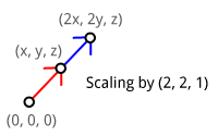
If you understand how the previous matrix was formed, it should not be difficult to come up with a matrix that scales a given vector by (SX,SY,SZ).

If you think about it for a moment, you can see that scaling would also be possible with a mere 3-by-3 matrix.

Rotation

A rotation transformation rotates a vector around the origin (0,0,0) using a given axis and angle. To understand how the axis and the angle control a rotation, let's do a small experiment.

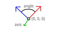
Put your thumb up against your monitor and try rotating your hand around it. The object, your hand, is rotating around your thumb: the rotation axis. The further you rotate your hand away from its initial position, the higher the rotation angle.

In this way the rotation axis can be imagined as an arrow an object is rotating around. If you imagine your monitor to be a 2-dimensional XY surface, the rotation axis (your thumb) is pointing in the Z direction.

Objects can be rotated around any given axis, but for now only the X, Y and Z axis are important. You'll see later in this chapter that any rotation axis can be established by rotating around the X, Y and Z axis simultaneously.

The matrices for rotating around the three axes are specified here. The rotation angle is indicated by the theta ($\theta$).

Rotation around X-axis:

Rotation around Y-axis:

Rotation around Z-axis:

Don't worry about understanding the actual geometry behind this, explaining that is beyond the scope of this guide. What matters is that you have a solid idea of how a rotation is described by a rotation axis and an angle and that you've at least seen what a rotation matrix looks like.

Matrix-Matrix product

In the previous section you've seen how transformation matrices can be used to apply transformations to vectors, but this by itself is not very useful. It clearly takes far less effort to do a translation and scaling by hand without all those pesky matrices!

Now, what if I told you that it is possible to combine as many transformations as you want into a single matrix by simply multiplying them? You would be able to apply even the most complex transformations to any vertex with a simple multiplication.

In the same style as the previous section, this is how the product of two 4-by-4 matrices is determined:

The above is commonly recognized among mathematicians as an indecipherable mess. To get a better idea of what's going on, let's consider two 2-by-2 matrices instead.

Try to see the pattern here with help of the colors. The factors on the left side (1,2 and 3,4) of the multiplication dot are the values in the row of the first matrix. The factors on the right side are the values in the rows of the second matrix repeatedly. It is not necessary to remember how exactly this works, but it's good to have seen how it's done at least once.

Combining transformations

To demonstrate the multiplication of two matrices, let's try scaling a given vector by (2,2,2) and translating it by (1,2,3). Given the translation and scaling matrices above, the following product is calculated:

Notice how we want to scale the vector first, but the scale transformation comes last in the multiplication. Pay attention to this when combining transformations or you'll get the opposite of what you've asked for.

Now, let's try to transform a vector and see if it worked:

Perfect! The vector is first scaled by two and then shifted in position by (1,2,3).

Transformations in OpenGL

You've seen in the previous sections how basic transformations can be applied to vectors to move them around in the world. The job of transforming 3D points into 2D coordinates on your screen is also accomplished through matrix transformations. Just like the graphics pipeline, transforming a vector is done step-by-step. Although OpenGL allows you to decide on these steps yourself, all 3D graphics applications use a variation of the process described here.

Each transformation transforms a vector into a new coordinate system, thus moving to the next step. These transformations and coordinate systems will be discussed below in more detail.

Model matrix

The model matrix transforms a position in a model to the position in the world. This position is affected by the position, scale and rotation of the model that is being drawn. It is generally a combination of the simple transformations you've seen before. If you are already specifying your vertices in world coordinates (common when drawing a simple test scene), then this matrix can simply be set to the identity matrix.

View matrix

In real life you're used to moving the camera to alter the view of a certain scene, in OpenGL it's the other way around. The camera in OpenGL cannot move and is defined to be located at (0,0,0) facing the negative Z direction. That means that instead of moving and rotating the camera, the world is moved and rotated around the camera to construct the appropriate view.

Older versions of OpenGL forced you to use ModelView and Projection transformations. The ModelView matrix combined the model and view transformations into one. I personally find it is easier to separate the two, so the view transformation can be modified independently of the model matrix.

That means that to simulate a camera transformation, you actually have to transform the world with the inverse of that transformation. Example: if you want to move the camera up, you have to move the world down instead.

Projection matrix

After the world has been aligned with your camera using the view transformation, the projection transformation can be applied, resulting in the clip coordinates. If you're doing a perspective transformation, these clip coordinates are not ready to be used as normalized device coordinates just yet.

To transform the clipping coordinate into a normalized device coordinate, perspective division has to be performed. A clipping coordinate resulting from a perspective projection has a number different than 1 in the fourth row, also known as w. This number directly reflects the effect of objects further away being smaller than those up front.

The x and y coordinates will be in the familiar -1 and 1 range now, which OpenGL can transform into window coordinates. The z is known as the depth and will play an important role in the next chapter.

The coordinates resulting from the projection transformation are called clipping coordinates because the value of w is used to determine whether an object is too close or behind the camera or too far away to be drawn. The projection matrix is created with those limits, so you'll be able to specify these yourself.

Putting it all together

To sum it all up, the final transformation of a vertex is the product of the model, view and projection matrices.

This operation is typically performed in the vertex shader and assigned to the gl_Position return value in clipping coordinates. OpenGL will perform the perspective division and transformation into window coordinates. It is important to be aware of these steps, because you'll have to do them yourself when working with techniques like shadow mapping.

Using transformations for 3D

Now that you know three important transformations, it is time to implement these in code to create an actual 3D scene. You can use any of the programs developed in the last two chapters as a base, but I'll use the texture blending sample from the end of the last chapter here.

To introduce matrices in the code, we can make use of the GLM (OpenGL Math) library. This library comes with vector and matrix classes and will handle all the math efficiently without ever having to worry about it. It is a header-only library, which means you don't have to link with anything.

To use it, add the GLM root directory to your include path and include these three headers:

#include <glm/glm.hpp>
#include <glm/gtc/matrix_transform.hpp>
#include <glm/gtc/type_ptr.hpp>

The second header includes functions to ease the calculation of the view and projection matrices. The third header adds functionality for converting a matrix object into a float array for usage in OpenGL.

A simple transformation

Before diving straight into 3D, let's first try a simple 2D rotation.

glm::mat4 trans = glm::mat4(1.0f);
trans = glm::rotate(trans, glm::radians(180.0f), glm::vec3(0.0f, 0.0f, 1.0f));

The first line creates a new 4-by-4 matrix and initializes it to the identity matrix. The glm::rotate function multiplies this matrix by a rotation transformation of 180 degrees around the Z axis. Remember that since the screen lies in the XY plane, the Z axis is the axis you want to rotate points around.

To see if it works, let's try to rotate a vector with this transformation:

glm::vec4 result = trans * glm::vec4(1.0f, 0.0f, 0.0f, 1.0f);
printf("%f, %f, %f\n", result.x, result.y, result.z);

As expected, the output is (-1,0,0). A counter-clockwise rotation of 180 degrees of a vector pointing to the right results in a vector pointing to the left. Note that the rotation would be clockwise if an axis (0,0,-1) was used.

The next step is to perform this transformation in the vertex shader to rotate every drawn vertex. GLSL has a special mat4 type to hold matrices and we can use that to upload the transformation to the GPU as uniform.

GLint uniTrans = glGetUniformLocation(shaderProgram, "trans");
glUniformMatrix4fv(uniTrans, 1, GL_FALSE, glm::value_ptr(trans));

The second parameter of the glUniformMatrix4fv function specifies how many matrices are to be uploaded, because you can have arrays of matrices in GLSL. The third parameter specifies whether the specified matrix should be transposed before usage. This is related to the way matrices are stored as float arrays in memory; you don't have to worry about it. The last parameter specifies the matrix to upload, where the glm::value_ptr function converts the matrix class into an array of 16 (4x4) floats.

All that remains is updating the vertex shader to include this uniform and use it to transform each vertex:

#version 150 core

in vec2 position;
in vec3 color;
in vec2 texcoord;

out vec3 Color;
out vec2 Texcoord;

uniform mat4 trans;

void main()
{
    Color = color;
    Texcoord = texcoord;
    gl_Position = trans * vec4(position, 0.0, 1.0);
}

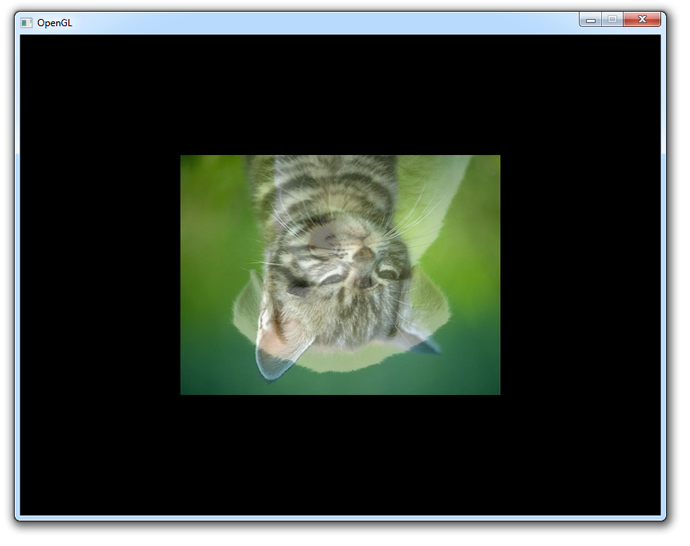
The primitives in your scene will now be upside down.

To spice things up a bit, you could change the rotation with time:

auto t_start = std::chrono::high_resolution_clock::now();

...

// Calculate transformation
auto t_now = std::chrono::high_resolution_clock::now();
float time = std::chrono::duration_cast<std::chrono::duration<float>>(t_now - t_start).count();

glm::mat4 trans;
trans = glm::rotate(
    trans,
    time * glm::radians(180.0f),
    glm::vec3(0.0f, 0.0f, 1.0f)
);
glUniformMatrix4fv(uniTrans, 1, GL_FALSE, glm::value_ptr(trans));

// Draw a rectangle from the 2 triangles using 6 indices
glDrawElements(GL_TRIANGLES, 6, GL_UNSIGNED_INT, 0);

...

This will result in something like this:

You can find the full code here if you have any issues.

Going 3D

The rotation above can be considered the model transformation, because it transforms the vertices in object space to world space using the rotation of the object.

glm::mat4 view = glm::lookAt(
    glm::vec3(1.2f, 1.2f, 1.2f),
    glm::vec3(0.0f, 0.0f, 0.0f),
    glm::vec3(0.0f, 0.0f, 1.0f)
);
GLint uniView = glGetUniformLocation(shaderProgram, "view");
glUniformMatrix4fv(uniView, 1, GL_FALSE, glm::value_ptr(view));

To create the view transformation, GLM offers the useful glm::lookAt function that simulates a moving camera. The first parameter specifies the position of the camera, the second the point to be centered on-screen and the third the up axis. Here up is defined as the Z axis, which implies that the XY plane is the "ground".

glm::mat4 proj = glm::perspective(glm::radians(45.0f), 800.0f / 600.0f, 1.0f, 10.0f);
GLint uniProj = glGetUniformLocation(shaderProgram, "proj");
glUniformMatrix4fv(uniProj, 1, GL_FALSE, glm::value_ptr(proj));

Similarly, GLM comes with the glm::perspective function to create a perspective projection matrix. The first parameter is the vertical field-of-view, the second parameter the aspect ratio of the screen and the last two parameters are the near and far planes.

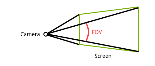
Field-of-view

The field-of-view defines the angle between the top and bottom of the 2D surface on which the world will be projected. Zooming in games is often accomplished by decreasing this angle as opposed to moving the camera closer, because it more closely resembles real life.

By decreasing the angle, you can imagine that the "rays" from the camera spread out less and thus cover a smaller area of the scene.

The near and far planes are known as the clipping planes. Any vertex closer to the camera than the near clipping plane and any vertex farther away than the far clipping plane is clipped as these influence the w value.

Now piecing it all together, the vertex shader looks something like this:

#version 150 core

in vec2 position;
in vec3 color;
in vec2 texcoord;

out vec3 Color;
out vec2 Texcoord;

uniform mat4 model;
uniform mat4 view;
uniform mat4 proj;

void main()
{
    Color = color;
    Texcoord = texcoord;
    gl_Position = proj * view * model * vec4(position, 0.0, 1.0);
}

Notice that I've renamed the matrix previously known as trans to model and it is still updated every frame.

Success! You can find the full code here if you get stuck.

Exercises

• Make the rectangle with the blended image grow bigger and smaller with sin. (Solution)
• Make the rectangle flip around the X axis after pressing the space bar and slowly stop again. (Solution)